iNaturalist Introduced Bubble Plot

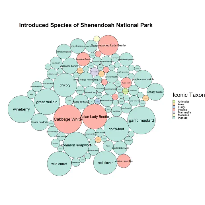
Code to make this figure is below and can be downloaded here: Change the place_id and the place_name to your place of interest. Find your place ID from the iNaturalist search function, when you search your location name in the search bar, like “Fairfax County”, the resulting url has the place name in the url (ex. for the url https://www.inaturalist.org/observations?place_id=738 the place name is 738)

	#install.packages("tidyverse", "devtools", "ggraph", "packcircles")
	#library(devtools)
	#devtools::install_github("hrbrmstr/curlconverter")

	library(curlconverter)
	library(tidyverse)
	library(ggraph)
	library(packcircles)

	place_id <- 744
	place_name <- "PWC"

	iconic_name <- NULL
	name <- NULL
	common <- NULL

	api <- paste("curl -X GET --header 'Accept: application/json' 'https://api.inaturalist.org/v1/observations?endemic=false&geo=true&introduced=true&place_id='", place_id, "&quality_grade=research&per_page=200&order=desc&order_by=created_at'", sep = "")
	my_ip <- straighten(api) %>% 
		make_req()
	dat <- content(my_ip[[1]](), as="parsed")
	for(i in 1:length(dat$results)){
	   iconic_name <- c(iconic_name, dat$results[[i]]$taxon$iconic_taxon_name)
	   name <- c(name,dat$results[[i]]$taxon$name)
	   if(is.null(dat$results[[i]]$taxon$preferred_common_name)){
		 common <- c(common, NA)}else{
		 common <- c(common, dat$results[[i]]$taxon$preferred_common_name)}
	}
	if (dat$total_results > 200){
	for (i in 2:floor(dat$total_results/200)){
	  api <- paste("curl -X GET --header 'Accept: application/json' 'https://api.inaturalist.org/v1/observations?endemic=false&geo=true&introduced=true&place_id='", place_id, "&quality_grade=research&page=", i, "&per_page=200&order=desc&order_by=created_at'", sep = "")
	  my_ip <- straighten(api) %>% 
		make_req()
	  dat <- content(my_ip[[1]](), as="parsed")
	  for(j in 1:length(dat$results)){
		iconic_name <- c(iconic_name, dat$results[[j]]$taxon$iconic_taxon_name)
		name <- c(name,dat$results[[j]]$taxon$name)
		if(is.null(dat$results[[j]]$taxon$preferred_common_name)){
		  common <- c(common, NA)}else{
		  common <- c(common, dat$results[[j]]$taxon$preferred_common_name)}
	  }
	}
	}


	dat2 <- dat
	dat2 <- data.frame(iconic_name,name,common)

	dat2 %>% 
	  group_by(common, iconic_name) %>%
	  summarise(n = n()) -> data
	names(data) <- c("group", "iconic", "value")

	packing <- circleProgressiveLayout(data$value, sizetype='area')
	data <- cbind(data, packing)
	dat.gg <- circleLayoutVertices(packing, npoints=50)
	dat.gg$group <- rep(data$iconic, each = 51)

	# Make the plot
	ggplot() + 
	  # Make the bubbles
	  geom_polygon(data = dat.gg, aes(x, y, group = id, fill=as.factor(group)), colour = "black", alpha = 0.6) +
	  # Add text in the center of each bubble + control its size
	  geom_text(data = data, aes(x, y, size=value, label = group)) +
	  scale_size_continuous(range = c(1,10), guide = F) +
	  # General theme:
	  theme_void() + 
	  theme() +
	  coord_equal() + 
	  ggtitle(paste("Introduced Species of", place_name)) +
	  scale_fill_brewer(palette="Set3", direction=-1) + 
	  theme(plot.title = element_text(size = 40, face = "bold")) + 
	  labs(fill = "Iconic Taxon") + 
	  theme(legend.text=element_text(size=20), legend.title = element_text(size=40))+
	  theme(plot.title = element_text(hjust = 0.5))

	ggsave(paste("introduced_species_of_", gsub(" ", "_", place_name), ".png", sep = ""), height = 25, width = 25)